General Vocabulary
Ballot: the information gathered from a voter, usually a ranking, but could be points as well.
Ballot generator: a method for creating ballots.
Bloc: a group of voters who share some similar voting patterns.
BLT: a file type used to record CVRs in Scottish elections.
Bullet vote: casting a vote for a single candidate.
CVR: cast vote record, i.e., the collection of ballots.
Election: a choice of rules for converting a preference profile into an outcome.
Linear ranking: an ordering of the candidates \(A>C>B\) by your preference for each. \(A>C\) means you prefer \(A\) to \(C\).
Preference profile: a collection of ballots from voters. Note, this is not the same as an election.
Ranked choice voting: the act of electing candidates using rankings instead of bullet votes.
Social choice theory: the study of making decisions from collective input.
Preference Intervals
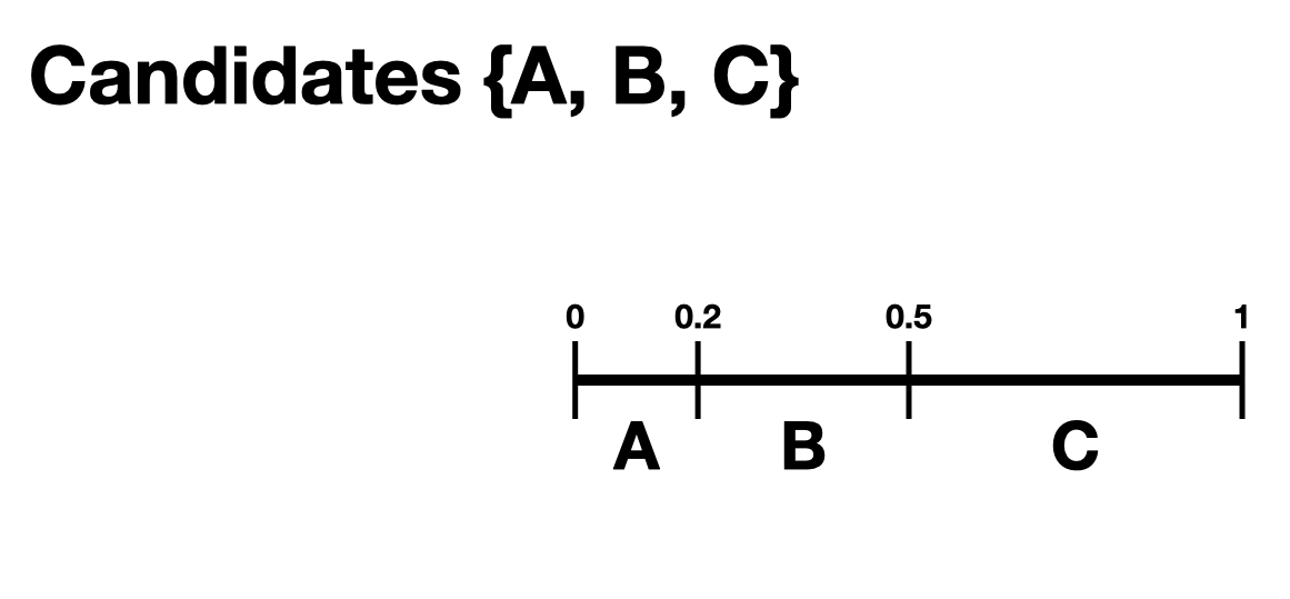
A preference interval stores information about a voter’s preferences for candidates. We visualize this, unsurprisingly, as an interval. We take the interval \([0,1]\) and divide it into pieces, where each piece is proportional to the voter’s preference for a particular candidate. If we have two candidates \(A,B\), we fix an order of our interval and say that the first piece will denote our preference for \(A,\) and the second for \(B\). As an abuse of notaton, one could write \((A,B)\), where we let \(A\) represent the candidate and the length of the interval. For example, if a voter likes candidate \(A\) a lot more than \(B\), they might have the preference interval \((0.9, 0.1)\). This can be extended to any number of candidates, as long as each entry is non-negative and the total of the entries is 1.
We have not said how this preference interval actually gets translated into a ranked ballot for a particular voter. That we leave up to the ballot generator models, like the Plackett-Luce model.
It should be remarked that there is a difference, at least to VoteKit, between the intervals \((0.9,0.1,0.0)\) and \((0.9,0.1)\). While both say there is no preference for a third candidate, if the latter interval is fed into VoteKit, that third candidate will never appear on a generated ballot. If we feed it the former interval, the third candidate will always appear at the bottom of the ballot.
VoteKit provides an option, from_params,
which allows you to randomly generate preference intervals. For more on
how this is done, see the page on Simplices.
Simplices in Social Choice
Candidate Simplex
There is a unique correspondence between preference intervals and points in the candidate simplex. This will be easiest to visualize with three candidates; let’s call them \(A,B,C\). Our candidate simplex is a triangle, with each vertex representing one of the candidates. If a point on the simplex is close to vertex \(A\), that means the point represents a preference interval with strong preference for \(A\) (likewise for \(B\) or \(C\)).
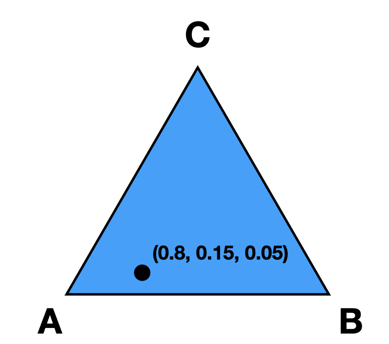
More formally, we have vectors \(e_A = (1,0,0), e_B = (0,1,0), e_C = (0,0,1)\). Each point on the triangle is a vector \((a,b,c)\) where \(a+b+c=1\) and \(a,b,c\ge 0\). That is, each point is a convex combination of the vectors \(e_A, e_B,e_C\). The value of \(a\) denotes someone’s “preference” for \(A\). Thus, a point in the candidate simplex is precisely a preference interval for the candidates!
The candidate simplex extends to an arbitrary number of candidates.
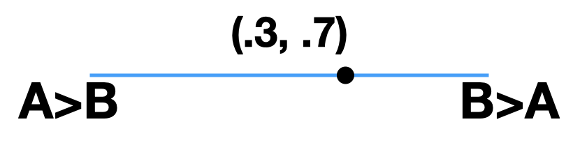
Ballot Simplex
The ballot simplex is the same thing as the candidate simplex, except
now the vertices of the simplex represent full linear rankings. So in
the case of 3 candidates, we have \(3!=6\) vertices, one for each
permutation of the ranking \(A>B>C\). A point in the ballot simplex
represents a probability distribution over these full linear rankings.
This is much harder to visualize since we’re stuck in 3 dimensions!
Here we present a visualization for two candidates.
Dirichlet Distribution
Throughout VoteKit, it will be useful to be able to sample from the candidate simplex (if we want to generate preference intervals) or the ballot simplex (if we want a distribution on rankings). How will we sample from the simplex? The Dirichlet distribution!
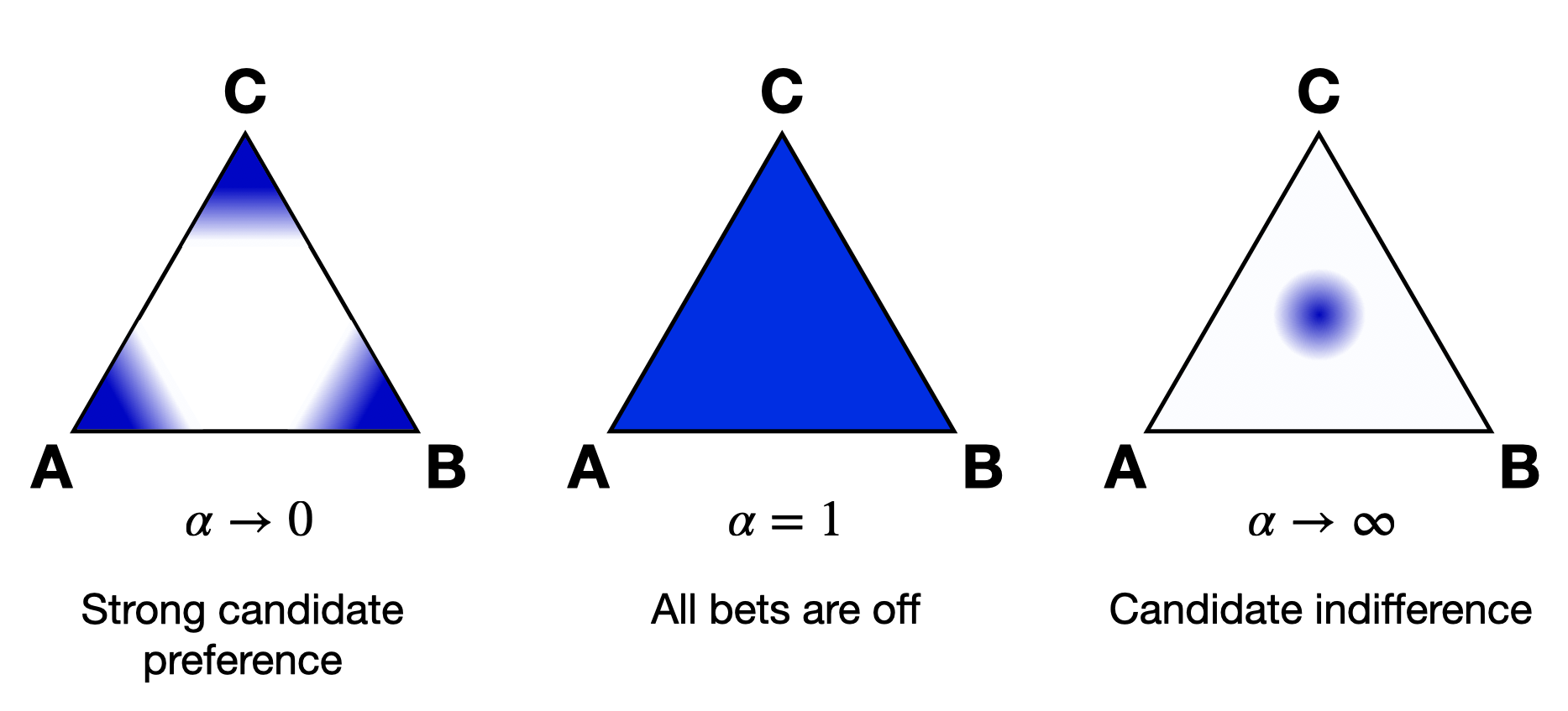
In what follows, we will presume we are discussing the candidate simplex, but it all applies to the ballot simplex as well. The Dirichlet distribution is a probability distribution on the simplex. We parameterize it with a value \(\alpha \in (0,\infty)\). As \(\alpha\to \infty\), the mass of the distribution moves to the center of the simplex. This means we are more likely to sample preference intervals that have equal support for all candidates. As \(\alpha\to 0\), the mass moves to the vertices. This means we are more likely to sample preference intervals that have strong support for one candidate. When \(\alpha=1\), all bets are off. In this regime, we have no knowledge of which candidates are likely to receive support.
The value \(\alpha\) is never allowed to be 0 or \(\infty\), so VoteKit uses an arbitrary large number (\(10^{20}\)) and an arbitrary small number \((10^{-10})\). When members of MGGG have done experiments for studies, they have taken \(\alpha = 1/2\) to be small and \(\alpha = 2\) to be big.
Multiple Blocs
Cohesion Parameters
When there are multiple blocs, or types, of voters, we utilize cohesion
parameters to measure how much voters prefer candidates from their own
bloc versus the opposing blocs. In our name models, like
name_PlackettLuce or name_BradleyTerry, the cohesion parameters
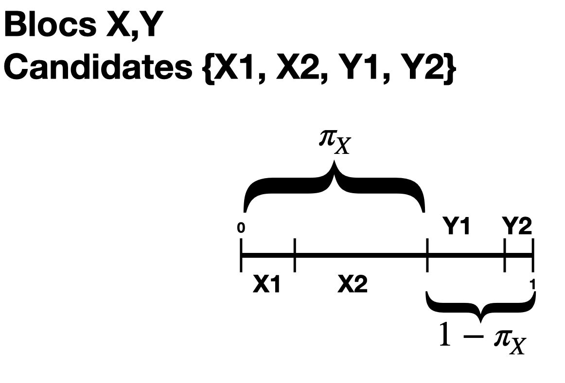
operate as follows. Suppose there are two blocs of voters, \(X,Y\).
We assume that voters from the \(X\) bloc have some underlying
preference interval \(I_{XX}\) for
candidates within their bloc, and a different underlying preference
interval \(I_{XY}\) for the candidates in the opposing bloc. Let \(\pi_X\) denote
the cohesion parameter for the \(X\) bloc.
In order to construct one preference interval for \(X\) voters, we take \(I_{XX}\) and scale it by \(\pi_X\), then we take \(I_{XY}\) and scale it by \(1-\pi_X\), and finally we concatenate the two. As a concrete example, if \(\pi_X = .75\), this means that 3/4 of the preference interval for \(X\) voters is taken up by candidates from the \(X\) bloc, and the other 1/4 by \(Y\) candidates. You can think about the cohesion parameter as measuring some tendency to prefer your own bloc over the others. A high level of cohesion indicates a strong preference for your own bloc, i.e. a polarized election.
In our slate models, like slate_PlackettLuce, the cohesion parameter
is used to determine the probability of sampling a particular slate at
each position in the ballot. How exactly this is done depends on the
model. Then candidate names are filled in afterwards by sampling without
replacement from each preference interval.
Combining Dirichlet and Cohesion
When there are multiple blocs of voters, we need more than one
\(\alpha\) value for the Dirichlet distribution. Suppose there are
two blocs of voters, \(X,Y\). Then we need four values,
\(\alpha_{XX}, \alpha_{XY}, \alpha_{YX}, \alpha_{YY}\). The value
\(\alpha_{XX}\) determines what kind of preferences \(X\) voters
will have for \(X\) candidates. The value \(\alpha_{XY}\)
determines what kind of preferences \(X\) voters have for \(Y\)
candidates. We sample preference intervals from the candidate simplex
using these \(\alpha\) values, and then use cohesion parameters to
combine them into a single interval, one for each bloc. This is how
from_params initializes different ballot
generator models.
Ballot Generators
In addition to being able to read real world voting data, VoteKit also has the ability to generate ballots using different models. This is useful when you want to run experiments or just play around with some data. We make no claims that these models accurately predict real voting behavior.
Ballot Simplex Models
Models listed below generate ballots by using the ballot simplex. This means we take a draw from the Dirichlet distribution, which gives us a probability distribution on full, linear rankings. We then generate ballots according to this distribution.
Impartial Culture
The Impartial Culture model has \(\alpha = \infty\). As discussed in the ballot simplex section, this is not actually a valid parameter for the Dirichlet distribution, so instead VoteKit sets \(\alpha = 10^{20}\). This means that the point drawn from the ballot simplex has a very high probability of being in the center, which means each linear ranking has a near-equal probability of being sampled.
Impartial Anonymous Culture
The Impartial Anonymous Culture model has \(\alpha = 1\). This means that the point that determines the distribution on rankings is uniformly drawn from the ballot simplex. This does not mean we have a uniform distribution on rankings; rather, we have the possibility of any distribution on rankings.
Candidate Simplex Models
Name-Plackett-Luce
The name-Plackett-Luce model (n-PL) samples ranked ballots as follows. Assume there are \(n\) blocs of voters. Within a bloc, say bloc \(A\), voters have \(n\) preference intervals, one for each slate of candidates. A bloc also has a fixed \(n\)-tuple of cohesion parameters \(\pi_A = (\pi_{AA}, \pi_{AB},\dots)\); we require that \(\sum_B \pi_{AB}=1\). To generate a ballot for a voter in bloc \(A\), each preference interval \(I_B\) is rescaled by the corresponding cohesion parameter \(\pi_{AB}\), and then concatenated to create one preference interval. Voters then sample without replacement from the combined preference interval.
Name-Bradley-Terry
The name-Bradley-Terry model (n-BT) samples ranked ballots as follows. Assume there are \(n\) blocs of voters. Within a bloc, say bloc \(A\), voters have \(n\) preference intervals, one for each slate of candidates. A bloc also has a fixed \(n\)-tuple of cohesion parameters \(\pi_A = (\pi_{AA}, \pi_{AB},\dots)\); we require that \(\sum_B \pi_{AB}=1\). To generate a ballot for a voter in bloc \(A\), each preference interval \(I_B\) is rescaled by the corresponding cohesion parameter \(\pi_{AB}\), and then concatenated to create one preference interval. Voters then sample ballots proportional to pairwise probabilities of candidates. That is, the probability that the ballot \(C_1>C_2>C_3\) is sampled is proprotional to \(P(C_1>C_2)P(C_2>C_3)P(C_1>C_3)\), where these pairwise probabilities are given by \(P(C_1>C_2) = C_1/(C_1+C_2)\). Here \(C_i\) denotes the length of \(C_i\)’s share of the combined preference interval.
Name-Cumulative
The name-Cumulative model (n-C) samples ranked ballots as follows. Assume there are \(n\) blocs of voters. Within a bloc, say bloc \(A\), voters have \(n\) preference intervals, one for each slate of candidates. A bloc also has a fixed \(n\)-tuple of cohesion parameters \(\pi_A = (\pi_{AA}, \pi_{AB},\dots)\); we require that \(\sum_B \pi_{AB}=1\). To generate a ballot for a voter in bloc \(A\), each preference interval \(I_B\) is rescaled by the corresponding cohesion parameter \(\pi_{AB}\), and then concatenated to create one preference interval. To generate a ballot, voters sample with replacement from the combined interval as many times as determined by the length of the desired ballot.
Slate-Plackett-Luce
The slate-Plackett-Luce model (s-PL) samples ranked ballots as follows. Assume there are \(n\) blocs of voters. Within a bloc, say bloc \(A\), voters have \(n\) preference intervals, one for each slate of candidates. A bloc also has a fixed \(n\)-tuple of cohesion parameters \(\pi_A = (\pi_{AA}, \pi_{AB},\dots)\); we require that \(\sum_B \pi_{AB}=1\). Now the cohesion parameters play a different role than in the name models above. For s-PL, \(\pi_{AB}\) gives the probability that we put a \(B\) candidate in each position on the ballot. If we have already exhausted the number of \(B\) candidates, we remove \(\pi_{AB}\) and renormalize. Once we have a ranking of the slates on the ballot, we fill in candidate ordering by sampling without replacement from each individual preference interval (we do not concatenate them!).
Slate-Bradley-Terry
The slate-Bradley-Terry model (s-BT) samples ranked ballots as follows. We assume there are 2 blocs of voters. Within a bloc, say bloc \(A\), voters have 2 preference intervals, one for each slate of candidates. A bloc also has a fixed tuple of cohesion parameters \(\pi_A = (\pi_A, 1-\pi_A)\). Now the cohesion parameters play a different role than in the name models above. For s-BT, we again start by filling out a ballot with bloc labels only. Now, the probability that we sample the ballot \(A>A>B\) is proportional to \(\pi_A^2\); just like name-Bradley-Terry, we are computing pairwise comparisons. In \(A>A>B\), slate \(A\) must beat slate \(B\) twice. As another example, the probability of \(A>B>A\) is proportional to \(\pi_A(1-\pi_A)\). Once we have a ranking of the slates on the ballot, we fill in candidate ordering by sampling without replacement from each individual preference interval (we do not concatenate them!).
Alternating-Crossover
The Alternating-Crossover model (AC) samples ranked ballots as follows. It assumes there are only two blocs. Within a bloc, voters either vote with the bloc, or they alternate. The proportion of such voters is determined by the cohesion parameter. If a voter votes with the bloc, they list all of their bloc’s candidates above the other bloc’s. If a voter alternates, they list an opposing candidate first, and then alternate between their bloc and the opposing until they run out of one set of candidates. In either case, the order of candidates is determined by a PL model.
The AC model can generate incomplete ballots if there are a different number of candidates in each bloc.
The AC model can be initialized from a set of preference intervals, along with which candidates belong to which bloc and a set of cohesion parameters.
The AC model only works with two blocs.
The AC model also requires information about what proportion of voters belong to each bloc.
Cambridge-Sampler
The Cambridge-Sampler (CS) samples ranked ballots as follows. Assume there is a majority and a minority bloc. If a voter votes with their bloc, they rank a bloc candidate first. If they vote against their bloc, they rank an opposing bloc candidate first. The proportion of such voters is determined by the cohesion parameter. Once a first entry is recorded, the CS samples a ballot type from historical Cambridge, MA election data. That is, if a voter puts a majorrity candidate first, the rest of their ballot type is sampled in proportion to the number of historical ballots that started with a majority candidate. Once a ballot type is determined, the order of candidates is determined by a PL model.
Let’s do an example. I am a voter in the majority bloc. I flip a coin weighted by the cohesion parameter, and it comes up tails. My ballot type will start with a minority candidate \(m\). The CS samples historical ballots that also started with \(m\), and tells me my ballot type is \(mmM\); two minority candidates, then a majority. Finally, CS uses a PL model to determine which minority/majority candidates go in the slots.
CS can generate incomplete ballots since it uses historical data.
The CS model can be initialized from a set of preference intervals, along with which candidates belong to which bloc and a set of cohesion parameters.
The CS model only works with two blocs if you use the Cambridge data.
The CS model also requires information about what proportion of voters belong to each bloc.
You can give the CS model other historical election data to use.
Spatial Models
1-D Spatial
The 1-D Spatial model samples ranked ballots as follows. First, it assigns each candidate a position on the real number line according to a normal distribution. Then, it does the same with each voter. Finally, a voter’s ranking is determined by their distance from each candidate.
The 1-D Spatial model only generates full ballots.
The 1-D Spatial model can be initialized from a list of candidates.
Elections
Ranking-based
Plurality/SNTV
Plurality or single non-transferable vote (SNTV). Winners are the \(m`\) candidates with the most first-place votes. As a system of election, this is equivalent to bloc plurality voting (see below), but this version is limited to one choice per voter and is read off of a ranked ballot rather than an approval ballot. It is also equivalent to limited voting when that system uses \(k=1\).
Borda
Positional voting system that assigns a decreasing number of points to
candidates based on order using a global score vector \((r_1,r_2,..,r_n)\). The conventional score
vector is \((n, n-1, \dots, 1)\), where n is the number of candidates.
A candidate in position 1 is given \(r_1\) points, a candidate in position 2 is given
\(r_2\), and so on. If a ballot is incomplete, the remaining points of the score
vector are evenly distributed to the unlisted candidates (see score_profile_from_rankings
function in utils). If a ballot has ties, the tied candidates are awarded an average of their
the scores over all possible completions of the tie.
The default for a Borda election is one winner – whoever has the highest point total – but
you can also use this Borda election method to elect multiple winners.
STV
STV stands for single transferable vote. Voters cast ranked choice ballots. A threshold is set; if a candidate crosses the threshold, they are elected. The threshold defaults to the Droop quota (defined below). We also enable functionality for the Hare quota.
In the first round, the first-place votes for each candidate are tallied. If a candidate crosses the threshold, they are marked “elected.” Any surplus votes for an elected candidate are distributed to the remaining candidates according to a transfer rule (all are transferred with fractional weight, by default). A further default specifies that multiple candidates over threshold can be simultaneously elected in a given round, as is the practice in Cambridge, MA; users have the option to opt for one-by-one election instead. If no candidate crosses threshold, the candidate with the fewest first-place votes is eliminated, and their ballots are fully redistributed according to the transfer rule. This repeats until all seats are filled. If too many ballots are exhausted for \(m\) candidates to cross threshold, then the top-positioned ones left at the end of the process fill out the seats.
The current transfer methods are stored in the
electionsmodule.
Quotas and Transfers for STV
Droop
If there are \(m\) seats up for election and \(N\) votes, the Droop quota is \(\frac{N}{m+1}+1\).
Hare
If there are \(m\) seats up for election and \(N\) votes, the Droop quota is \(\frac{N}{m}+1\).
Fractional Transfer
Under fractional transfer, all ballots that can be transferred (i.e., those with a next ranking specified) are assigned a new weight according to the share of votes for the elected candidate that were in excess of the threshold. For instance, if the threshold is 1000 votes and the candidate received 1500, their votes are transferred with 1/3 weight.
Random Transfer
Under random transfer, if there are \(S\) surplus votes for the winning candidate, \(S\) ballots are chosen uniformly at random to (fully) transfer, rather than transferring all ballots with fractional weight.
IRV
Instant runoff voting (IRV); An STV election for one seat. (This is intentionally redundant with STV, \(m=1\).) This system is widely practiced around the U.S.
SequentialRCV
An STV election in which votes are not transferred after a candidate has reached threshold, or been elected. This system is actually used in parts of Utah.
Alaska
Election method that first runs a Plurality election to choose a user-specified number of final-round candidates, then runs STV to choose \(m\) winners.
TopTwo
Eliminates all but the top two plurality vote-getters, and then conducts a runoff between them, reallocating other ballots.
DominatingSets (Smith method)
A “dominating set” is any set \(S\) of candidates such that everyone in \(S\) beats everyone outside of \(S\) head-to-head. The top tier (which is well defined) is often called the “Smith set,” and if it is just one person, they are called the “Condorcet candidate.” The Smith method of election declares the Smith set to be the winners, which means that users do not get to specify the number of winners.
Condo Borda
Just like Smith method, but user gets to choose the number of winners, \(m\). Ties are broken with Borda scores.
Score-based
Rating (score or range voting)
To fill \(m\) seats, voters score each candidate independently from \(0-L\), where \(L\) is some user-specified limit. The \(m\) winners are those with the highest total score.
Cumulative
Voters can score each candidate, but have a total budget of \(m\) points, where \(m\) is the number of seats to be filled. Spending all your points on one candidate is called “plumping” the vote. Winners are those with highest total score.
Limited
Just like cumulative voting, except total score must sum to no more than a user-specified \(k\), which is assumed strictly less than \(m\). (This is why it’s called “limited.”)
Approval-based
Approval
Standard approval voting lets voters choose any subset of candidates to approve. Winners are the \(m\) candidates who received the most approval votes.
Bloc Plurality
Like approval voting, but there is a user-specified limit of \(k\) approvals per voter. Most commonly, this would be run with \(k=m\).
Distances between PreferenceProfiles
Earthmover Distance
The Earthmover distance is a measure of how far apart two distributions
are over a given metric space. In our case, the metric space is the
BallotGraph endowed with the shortest-path metric. We then consider a
PreferenceProfile to be a probability distribution that weights each node (ballot) by the share
of the profile consisting of that ballot. Informally, the Earthmover distance considers “transportation plans”
that move mass from one distribution to the other; the cost of moving weight is the mass times the
graph distance moved. The distance between two distributions is minimum cost of a plan that moves
all mass from one to the other. For a more formal definition, see this wiki.
\(L_p\) Distance
The \(L_p\) distance is a family of metrics parameterized by \(p\in (0,\infty]\). It is computed as \(d(P_1,P_2) = \left(\sum |P_1(b)-P_2(b)|^p\right)^{1/p}\), where the sum is indexed over all possible ballots, and \(P_i(b)\) denotes the number of times that ballot was cast in profile \(i\). For a more formal discussion of \(L_p\) distance, see here.